Beef consumption in Indonesia tends to increase. National beef production is smaller than the demand for beef in Indonesia. So that to meet domestic meat consumption, beef imports are carried out. Importing countries need to pay attention to price volatility because if the price volatility of a commodity is high, it will have a bad impact on the importer. Therefore, the movement of meat prices in the global market needs to be understood by the government. This study aims to analyze the volatility of beef prices in the global market. The data used in this study is secondary monthly time series data from January 1960 to December 2020 from the World Bank's Pink Sheet Data. Beef price volatility analysis using ARIMA and ARCH-GARCH methods. The results showed that the highest volatility in beef prices occurred during the global economic recession in 2020. This volatility occurred at the beginning of the Covid-19 pandemic, which had an impact on cattle production disturbances, but demand continued to even tend to rise, resulting in high price volatility. Local cattle production needs to be increased to reduce imports so that they are resistant to turmoil in the global market.
Beef is a strategic food commodity, especially in Indonesia. Public interest is quite high for beef commodities. People are increasingly aware of the need for animal protein. This makes beef ranks second after poultry as a source of animal protein [1]. The demand for beef will certainly continue to increase along with the increase in population.
The price of beef fluctuates quite a bit from period to period. This fluctuation will greatly affect many parties, namely producers, consumers and small-scale beef processing industries. Changes in beef prices that occur in one market will have an impact on other markets and can be used to determine the strength of a market [2]. The availability of beef must continue to be considered. Currently, the national beef production is still unable to meet domestic beef needs. This encourages the import of beef from the global market. So that global beef prices need to know the upward trend. According to Sumaryanto [3], economic development and socio-political stability of a country require stable food prices.
Beef prices that are difficult to predict and continue to increase indicate that there is a volatile or fluctuating price trend. Volatility in this case refers to conditions that are unstable, varied and difficult to predict [4]. Price fluctuations can cause high price volatility [5]. In addition, the large or small volatility value shows how much the level of risk will be faced in the future [6]. Selection of the right policy by the government needs to be done so that people can continue to make purchases of beef. Therefore, sufficient information about global beef prices is needed. This is related to policies that will be made related to beef. Fluctuations in world beef prices have not been able to explain the actual situation, therefore it is necessary to analyze the volatility of beef prices in the global market. So that the right policies and decisions can be made. Given the many economic turmoils that have occurred in various parts of the world, such as the 1973 crisis, the 2008 crisis and the 2020 recession, it is necessary to know more about the state of beef prices in the global market in the face of these challenges. This study aims to analyze the volatility of beef prices in the global market.
Data Collection
This study uses secondary data in the form of monthly time series from January 1960 to December 2020. Data obtained from the World Bank's Pink Data Sheet.
Data Analysis
Autoregressive Integrated Moving Average (ARIMA) and Autoregressive Conditional Heteroscedasticity- Generalized Autoregressive Conditional Heteroscedasticity (ARCH GARCH) models were used to
identify beef price volatility. Data testing is carried out in several stages. The stages include:
Identify the ARCH effect
Estimation Model
Evaluation Model
ARCH GARCH Model
The ARCH model used in this study are:

The GARCH model in this study is as follows:

Information

Table 1: Heteroscedasticity Problem Identification Test
| ACF Value | Lag 1-15 prob | Kurtosis Value | Heteroscedasticity Problem |
| Not close to zero | Significant | 3,054 | Have |
Table 2: Results of Augmented Dickey Fuller Test
| ADF test level | ADF test first differencing |
| T-statistics | T-statistics |
| -1,265 | -14,539*** |
***) significant at 1 percent
Table 3: ARCH Effect Test Results
| The best ARIMA models | F statistics |
| ARIMA (1, 1, 1) | 135,733*** |
Table 4 Model Sufficiency Test Results
| Commodity | ARCH-LM test probability |
| Beef | 0,9497 |

Figure 1: Global Beef Price Volatility Chart
Model Identification
The data obtained were then performed data analysis. The identification of the model is the first thing that must be done. This identification aims to see the problem of heteroscedasticity by using the correlogram test and kurtosis test. The correlogram test can be seen from the value of the Autocorrelation Function (ACF) in the first 15 lags. If the ACF value is not close to zero, then the data has heteroscedasticity. Furthermore, the kurtosis value is also used to identify the problem of heteroscedasticity. If the kurtosis value is more than 3 then the data is heteroscedasticity.
Based on the results of the correlogram test in Table 1, it can be seen that the beef price data in this study has an ACF value that is not close to zero so that it has fulfilled the requirements needed for volatility analysis because it has heteroscedasticity problems. While the kurtosis value of beef price data in this study was 3.054, which means it was greater than 3, then the data had heteroscedasticity problems. Based on the correlogram test and kurtosis test, the data in this study has a heteroscedasticity problem. If the heteroscedasticity requirements have been met, the next stage of analysis can be carried out.
Model Estimation
After the heteroscedasticity conditions are met, the next thing to do is to estimate the ARIMA model. Stationary test using Augmented Dickey Fuller (ADF) is the first thing to do in forming the ARIMA model. If the probability value is less than the 5 percent significance level, it can be concluded that the data is stationary. If the data is still not stationary, differencing will continue until the data becomes stationary. To find out the best ARIMA model, it is done tentatively. The differencing value can describe the d value in the ARIMA model, while the AR (p) and MA (q) values are determined in a tentative way to produce the best ARIMA.
Based on Table 2, it can be seen that beef is not stationary at the 5 percent level of significance. So that the next stationary test is carried out, namely at the first difference stage. The beef data was stationary after the first differencing, so the beef commodity was stationary at the first difference. So it can be continued to find out the best ARIMA model. Based on these results, the value of d is obtained by 1. The values of p and q are determined tentatively. The best ARIMA of beef commodities obtained tentatively is as follows ARIMA (1, 1, 1). After the best ARIMA model is formed, then the ARCH test is carried out which is used to determine the ARCH effect in the ARIMA model that is formed. If the ARCH effect in the model is known, it can be continued to the ARCH GARCH test. The ARCH effect can be seen from the probability value of F statistic which is less than the alpha value of 0.05.
Based on Table 3, the ARIMA model of beef commodities has an ARCH effect so that it can be continued to test the best ARCH GARCH model. Based on the results of the analysis, the best ARCH GARCH model for beef commodities is GARCH (1,2).
Model Evaluation
After identifying the model and model estimation, the next step is model evaluation. In this study, the ARCH LM test was used to determine the ARCH effect was still present in the ARCH GARCH model. If the ARCH effect is no longer in the model, the model is good.
Based on Table 4, the results of the ARCH LM analysis show that the ARCH LM test results obtained are 0.9497. The probability value obtained is greater than the 0.05 level of significance. This shows that the selected model is free from the ARCH effect. So that the resulting model is adequate and meets fulfillet.
ARCH GARCH Model
After the stages to form the model are complete, the ARCH GARCH model of beef is obtained as follows:
Here is the GARCH (1,2) model of beef prices in global markets:
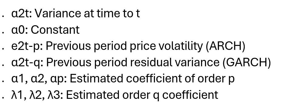
σ2t = 0.00031700604709 + 0.469892802485 e2t-1 + 0.227761279984 σ2t-1 + 0.375790624267 σ2t-2
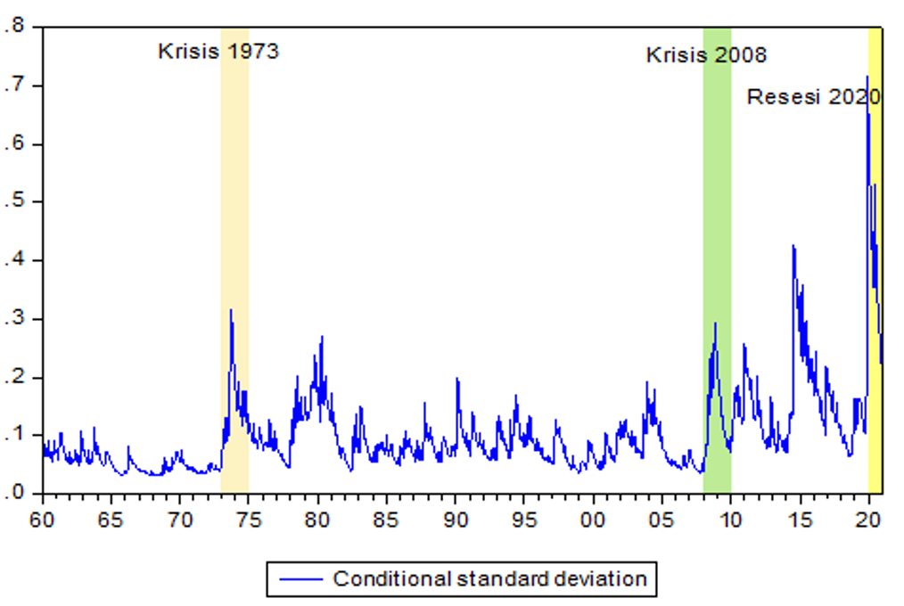
Based on table 4, it can be seen that the beef variance model equation has one ARCH term and two GARCH terms. Furthermore, it can be seen that the variance of beef prices in the world market is influenced by the volatility of beef prices in the previous period. The two GARCH coefficients when added together are 0.604, indicating that the variance shock will affect the price variance in the long term. The conditional standard deviation graph can be used to determine the volatility analysis. The higher the peak of the graph, the more volatile the commodity price will be. The following is a graph of global beef price volatility.
In this study, it is divided into 3 periods, namely the 1973 crisis, the 2008 crisis and the 2020 recession. This is because during these periods there were shocks in the economy. Figure 1 shows a graph of global beef price volatility during the period January 1960 to December 2020. High price volatility can be seen from the high peak of the graph. Beef prices in the 1973 crisis and the 2008 global crisis seemed more stable and less volatile. So it can be seen that the 1973 crisis and the 2008 crisis did not have an effect on global beef prices. Prices in the 1973 crisis and 2008 crisis remained stable because domestic and international supplies were still sufficient so that supply and demand were met. But what is of concern is that the highest volatility occurs in the 2020 recession, namely during the Covid-19 pandemic that spreads in various parts of the world. This is due to production disruptions from exporting countries which are constrained by cattle production due to certain policies during the Covid-19 pandemic. The imbalance between supply and demand causes prices to rise.
Beef prices in the 1973 crisis and 2008 crisis were not volatile and tended to be stable. The highest volatility in beef prices occurred in the 2020 recession. The Covid-19 pandemic caused beef prices to have high volatility. This is because there is an imbalance between supply and demand so that the price of beef increases sharply. Beef offers continue to decrease due to constraints in beef production due to the pandemic. Meanwhile, the demand for beef remains high, so prices have increased sharply.
Recommendations
National beef production has not been able to meet domestic meat needs, so imports must be carried out to fulfill it. So that beef prices in the global market, which have high volatility in the 2020 recession, need to be watched out for. The adequacy of domestic production can be met by increasing domestic beef production to reduce dependence on imports so that turmoil in the global market can be overcome.
Rusdiana, S. and A. Maesya. "Pertumbuhan Ekonomi dan Kebutuhan Pangan di Indonesia." Agriekonomika, vol. 6, no. 1, 2017, pp. 12–25.
Komalawati, Ratna W.A. et al. Volatilitas dan Transmisi Harga Daging Sapi di Indonesia: Studi Kasus di Jakarta, Bandung, Semarang dan Surabaya. Buletin Ilmiah Litbang Perdagangan, vol. 15, no. 1, 2021.
Sumaryanto. "Analisis Volatilitas Harga Eceran Beberapa Komoditas Pangan Utama dengan Model ARCH/GARCH." Jurnal Agro Ekonomi, vol. 27, no. 2, 2009, pp. 135–163.
Dewi, I. et al. "Price volatility analysis in indonesian beef market." Paper presented at 2nd International Conference on Sustainable Agriculture and Food Security: A Comprehensive Approach, Universitas Padjadjaran, Bandung, 2017.
Pipit, Yudi S.P. and Evahelda. "Analisis volatilitas harga daging sapi di provinsi kepulauan bangka belitung." Jurnal Ekonomi Pertanian dan Agribisnis (JEPA), vol. 3, no. 3, 2019, pp. 619–630.
Burhani, F.J. et al. "Analisis Volatilitas Harga Daging Sapi Potong dan Daging Ayam Broiler di Indonesia." Forum Agribisnis, vol. 19, no. 40, 2013.