The economies of developed countries are often overwhelmed by fears of high inflation rates as well as turbulent economic cycles. Meanwhile, in several developing countries, the economy had experienced growth but, in the end, it was not sustainable and was marked by high volatility in financial markets and also sometimes experienced an economic crisis caused by several factors [1-3]. In the end, several discussions led to the impact of the normalization of monetary policy and a growing market economy in uncertainty that posed a challenge to future growth. The impact of very high uncertainty values ​​causes economists to face great challenges in understanding the origins of economic uncertainty and analyzing the causal impact on the real economy [4-5]. Unexpected increases in uncertainty have a detrimental effect on the real economy and financial markets, with even greater quantitative impact during recessions [6-7].

Global economic uncertainty relates to the financial uncertainty generated by volatile international capital flows with maturities on the balance sheets of non-financial firms to increase the volatility of output, investment, and total factor productivity (TFP) in emerging market economies [8]. One potential trigger for global uncertainty as a simultaneous impact on national levels of uncertainty is oil, commodity and asset price shocks, or asynchronous shift in investor sentiment that may be related to changes in global perceptions of financial, economic or political risk [9-11].  High global uncertainty occurred in 2017 apart from political factors, namely the inauguration of US President Donald Trump, as well as the problem of global economic uncertainty due to the increase in interest rates of the United States, the Fed, and Britain's exit from Europe or Britain Exit (Brexit) thus creating uncertainty. the global economy [12].

We also collect evidence that the COVID-19 pandemic that occurred at the end of 2019 has continuously caused global economic conditions to decline. This phenomenon is made clear by the rising unemployment rate and the severity of the economic contraction relative to the size of the death   shock. The  unprecedented scale and nature of the COVID-19 crisis helps explain why it has resulted in such a tremendous spike in economic uncertainty [13].

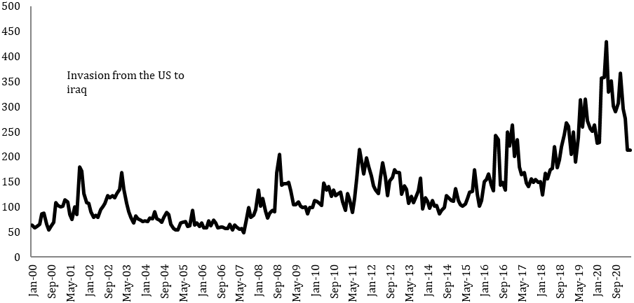
Figure 1: Developments of the global economic policy uncertainty index for the year 2000-2021

Source: http://www.policyuncertainty.com/index.html, 2021

The relationship between international economic shocks and macroeconomic conditions in developing countries needs to be analyzed more deeply, especially those related to the application of international monetary to the financial sector which affects the stability of monetary aggregate and exchange rate stability [14-15]. This study focuses on the influence of financial market volatility and global economic uncertainty on monetary policy in ASEAN 3, namely Indonesia, Thailand and the Philippines, which still have a puzzle. The selection of the scope is supported by the similarities in managing the economy, especially on exchange rate stability. Based on the phenomenon of inflation and exchange rates in monetary policy, Morgan [16] explained that the Asian financial crisis showed the importance of exchange rate flexibility and a high credibility policy framework, thereby increasing the independence of the central bank in determining inflationary policies and a more flexible exchange rate.

Based on global phenomena that influence economic fluctuations in several countries, this study wants to know the dynamics of monetary policy in ASEAN 3, namely Indonesia, the Philippines and Thailand. This analysis is based on the similarity of the exchange rate regime in ASEAN 3 and also the similarity in the implementation of monetary policy that leads to the inflation target to maintain economic stability. The Framework price stability policy applied in Indonesia, the Philippines, and Thailand is the Inflation Targeting Framework (ITF). In general, ITF is a monetary policy framework for a country's central bank through interest rate policy in setting inflation targets and achieving price stability and low inflation [17].

The international business cycle is an economic cycle that involves trade activities, labor activities, activities in the capital market, especially the development of the financial sector as well as relations with foreign financial activities such as foreign exchange [18-19]. The financial sector is not only focused on capital inflows and outflows but also currency trading activities between countries involving the main money markets in the world. International business activities are inseparable from the possibility of economic uncertainty and volatility from macroeconomic and monetary developments. Global uncertainty is one of the triggers for a country's economic growth to become unstable. This uncertainty triggered a reversal of foreign capital and a broad appreciation of the US dollar exchange rate, thereby contributing to pressure on global currency exchange rates[20-21], particularly in countries in the Emerging Market, including Indonesia.

This research focuses on the relationship between monetary policy on monetary aggregate and exchange rates in ASEAN 3 countries. The type of data used is secondary data obtained from the Asian Development Bank and International Financial Statistics with a period of 2006Q1-2020Q3. The object of the research was carried out in three parts of ASEAN countries, namely the Philippines, Indonesia, Thailand. The selection of the timeframe for the election from 2006Q1-2020Q3 was due to wanting to see the economic condition in a timeframe of 14 to see the moment that occurred because there was an economic crisis phenomenon that caused volatility in financial markets and global economic uncertainty that had an impact on the economic business cycle of developed countries and developing countries. developments, such as fluctuations in oil prices, the subprime mortgage crisis, the European crisis, the trade war between the US and China and other global economic turmoil such as the economic turmoil caused by the COVID-19 pandemic. The data used are M2 data, CPI, INT DIFF, exchange rates, real     GDP,    VIX,    GEPU    in      ASEAN       countries   3.

Table 1: Definition of research variable

The research method used in this study is the VAR Panel (Vector Autoregression). VAR is a model that can analyze the interdependence of variable time series, but it is different from the simultaneous equation model. VAR is a calculation time series econometric to see multivariable [22]. The reason for using the VAR method is because it is an effective method in macroeconomic modelling, time series and forecasting, although there are several weaknesses. The disadvantages of VAR are weight parameterization with the number of quadratic series and quickly finding degrees of freedom, but the advantages are that it produces more accurate estimates [23]. In the description, it is assumed that in the model there are endogenous (Y_t) and exogenous (X_t) variables, these variables may be at the level or 1st differences, depending on the data used with the assumption that there is no cointegration.

In general, the VAR model takes the form:

(1)

where is the element vector of the consumer price index, real gross domestic product, log nominal exchange rate, the difference between domestic interest rates and US 3-month treasury bills, volatility index, global economic policy uncertainty index.  is the vector constant nx 1. Is the coefficient of while n is the length of the lag. is a vector of shock for each variable.

The specifications of the research model are derived from previous studies, namely Ojede and Lam and Kohlscheen [24], so the research model in this study is as follows:

(2)

Panel data requires a root test, namely through the ADF test consisting of the Levin, Lin and Chu (LLC) test, Im, Pesaran and Shin (IPS) test. In econometric analysis, namely balanced panels (the same number of units for each individual) and unbalanced panels (different number of units of time for each individual [22].

Data Stationarity Test Results 

The data stationarity test known as the unit root test in this study is a pre-estimated test before proceeding to the VAR estimation test. The stationarity test of the data serves to avoid blunt regression [22,25]. Stationarity analysis on panel data uses several approaches, namely Levin, Lin, Chu (LLC), Im Pesaran, Shin (IPS), Augmented Dickey-Fuller Fisher-(F-ADF), and Fisher-Phillip Perron (Fisher-PP). Based on Table 2, the results show that the LogM3 variable in the LLC, ADF-Fisher and PP-Fisher method is stationary at the level, while in the IPS approach it is stationary at the level 1st difference. The stationarity of CPI data shows stationary at the level for the four methods, namely LLC, IPS, ADF-Fisher and PP-Fisher with a probability value of 0.0000.

Based on the results of the stationarity of the panel data, it can be seen that the RGDP of the LLC method is stationary at the level 1st difference, while it is stationary at the level of the IPS, ADF-Fisher and PP-Fisher methods. The NER variable is stationary at the level 1st difference in all methods. Furthermore, for the stationary VIX variable at the levels in all methods as evidenced by the probability < alpha 0.05. Meanwhile, for the stationary GEPU variable at the level 1st difference, the LLC, IPS, ADF-Fisher and PP-Fisher methods are used. Based on the results of data stationarity, it can be concluded that data that is not stationary at the same level, namely at the level, needs to be differentiated.

Cointegration Test Analysis Results 

This test aims to test the stationary of the residuals so that there is   an   adjustment  towards   a   long-term   balance between the variables that are the object of research. In this study, the Kao Residual Cointegration approach is used to detect the presence or absence of cointegration between panel data. Based on Table 3, shows that there is cointegration between variables as evidenced by a p-value smaller than a=5%. Cointegration corrects variable fluctuations in the short term towards stability in the long-term balance. 

Table 2: Results of the panel data stationarity

Probability, *Level level, **Level 1^st, ***Level 2^sd

Table 3: Results of the Kao Residual Cointegration Approach

Table 4: Result of optimum lag test 

Table 5: Result of stability test

Optimum Lag Test Results

This stage shows the optimum lag test results for ASEAN 3 panel data. Lag testing can use several approaches such as Likelihood Ratio (LR), Final Prediction Error (FPE), Akaike Information Criterion (AIC), Schwarz Information Criteria (SC).), and Hannan Quinn (HQ). In this study, the criteria for using lag use the Akaike Information Criterion (AIC). The purpose of the lag test is to determine the influence of a variable with past variables and with other endogenous variables within a certain period. Based on the results of the optimum lag test in Table 4, it can be seen that the lag length used for the next estimation is lag 6 with an absolute value of 34,63040.

Stability Test Results

Based on the data stability test results state that the model used is stable. This statement is evidenced by the modulus range with an average value of less than 1. The model stability test aims to test the validity of IRF and VD, thus the results of IRF and VD are valid.

Estimation Results 

The results of the estimation analysis of the VAR model show a significant effect between the independent variables on the dependent variable by looking at the probability value of t-statistics. The M3 variable has a significant effect on the variable itself at lag 4 with a significance value of less than 5% alpha with a positive coefficient value and at lag 6 with a significance value of less than 10% alpha with a negative coefficient. Furthermore, the CPI variable has no significant effect on the development of M3 as evidenced by a significance value of more than 5% and 10% in all lags. Furthermore, the RGDP variable has a significant effect on M3 at lag 2 with a significant value of less than 5% alpha with a positive coefficient value. These results indicate that each one percent increase in RGDP in the previous second period will significantly affect M3 growth for the current year. Bozkurt [26] explains that to reduce the risk of a deficit, then by developing a strategy based on economic growth, especially moving the real sector.

The NER variable shows a significant effect on lag 1 and lag 4 with a significance value of less than 5% alpha with a negative coefficient value. These results indicate that any depreciation of the exchange rate in ASEAN 3 by one percent in the previous first period and the previous fourth period can cause a significant decline in M3 in the current year. Abdullah et al. [27] explains that there is a significant negative relationship between the exchange rate and monetary aggregate in the short term. When a country experiences currency depreciation, it will have an impact on financial performance and economic growth, including the stability of the monetary aggregate which decreases.

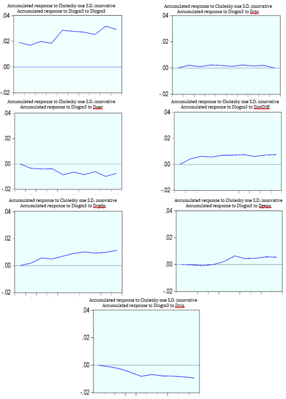
Figure 2: Result of Impulse responses function

Table 6: Result of VAR-P analysis

* Significant 5% ** Significant 10%

Table 7: Results of variance decomposition

because this is related to capital outflow. Meanwhile, the INTDIFF variable has a significant effect on lag 1 with a significance value of less than 5% alpha with a positive coefficient value. These results indicate that any increase in the differential interest rate by one percent in the previous first period will significantly affect M3 growth for the current year. The relationship between M3 and interest rates is explained by a review of Bank Indonesia [28] that raising interest rates can maintain the attractiveness of the domestic financial market, thereby strengthening Indonesia's external resilience in high global uncertainty.

M3 is significantly affected by the VIX variable at lag 4 with a significance value of less than 5% alpha and lag 5 with a significance value of less than 10% alpha with a positive coefficient value. These results indicate that any 1 percent increase in financial market volatility in the previous fourth and fifth periods will significantly affect M3 growth for the year. This condition proves that volatility in the financial market will affect the monetary and banking sectors of a country and the high level of competition    so that  the   economic balance of a country including emerging market countries, experiences shocks. The GEPU variable has a significant effect on M3 at lag 5 with a significance value of less than 5% alpha with a positive coefficient value. These results indicate that any 1 percent increase in global economic uncertainty in the previous fifth period will significantly affect M3 growth for the current year. Beckmann and Czudaj [29] research results suggest that there is a relationship between economic uncertainty and the growth of monetary aggregate.

IRF test results show a picture of how the response of a variable in the future if there is a disturbance in one other variable. If the impulse response graph shows a movement that is getting closer to the equilibrium point or returns to the previous balance, it means that the response of a variable due to a shock is increasingly disappearing so that the shock does not leave a permanent effect on the variable. Based on the results of the analysis using the IRF approach, the response of the LOGM3 to the shock variable itself in each period is quite large with a positive trend with the highest response in period 9 with a based point of 0.032. Furthermore, the LOGM3 response to the CPI shock showed a positive trend approaching the equilibrium point and returned to the equilibrium point in the 10th period.

The accumulation of LOGM3 responses to the RGDP shock at the beginning of the period was at the equilibrium point and subsequently showed an increased response with a positive trend with the highest response value in the 10th period with a base point of 0.011. while the LOM3 response to exchange rate shocks at the beginning of the period was at the equilibrium point and    subsequently    showed   a      negative   response.

Indifferent interest rate shocks are responded positively by LOGM3, which initially is at the equilibrium point and the next period shows a positive response and moves away from the equilibrium point. Furthermore, the LGM3 response to volatility index shocks shows a negative trend and, in each period, shows a response that is away from the equilibrium point. The M3 response to the GEPU shock in the initial period was at the equilibrium point and, in the 2nd, and 3rd periods it showed a negative response. The M3 response to the GEPU shock returned to its equilibrium point in the 4th period and subsequently showed an increased response with a positive trend.

Variance decomposition is used to compile forecast error variance of a variable, that is, how big is the difference between the variance before and after the shock. The shock in question comes from the relevant variable and other variables to see the relative influence between research variables. Based on the results of the analysis of variance decomposition, the variable that has the largest contribution to fluctuations in the M3 variable in period 4 is the M3 variable itself at 84.57%, the second-order is the shock from the INTDIFF variable at 4.73%, and then influenced by shocks to the RGDP variable of 3.93%, NER 2.74%, VIX 2.32%, CPI 1.51% and finally the smallest contribution by GEPU variable is 0.30%. But in the long term, namely, in the 10th period, the M3 variable shocks itself resulted in M3 fluctuations of 73.61%, the second order was shocks from the NER variable of 9.51%, and then M3 fluctuations were influenced by GEPU variable shocks of 4.19%, RGDP is 4.16%, INTDIFF is 3.68%, VIX is 3.05% and the last contribution is the smallest by the CPI variable at 1.79%.

The slowdown in economic growth that occurred in several developing countries was the impact of global uncertainty stemming from economic shocks in developing countries. progress as well as increasing market volatility. In addition, there are concerns about global dynamics stemming from the trade war in industrialized countries as well as the uncertainty of policies that will be implemented by developed countries which have an impact on monetary shocks in the ASEAN region. Based on the results of the discussion that has been described previously, it provides an answer that global economic uncertainty and financial market volatility have an influence on monetary policy in the ASEAN 3 region, namely Indonesia, the Philippines and Thailand.

Several global challenges that will have an impact on global economic growth are apart from the impact of the economic crisis, uncertainty in global oil prices and global commodity prices, which also stems from the normalization of US monetary policy and the trade war between developed countries such as the US-China as well as the COVID-19 pandemic. 19 which also threatens the condition of the world economy. Several of these phenomena have led to increased volatility in world financial markets, which in turn has an impact on the weakening of market exchange rates. One of the risks faced by Indonesia due to increased financial market volatility is a significant depreciation of the Rupiah, an increase in refinancing costs, insufficient hedging of debt in foreign currencies and a decline in profit margins which weakened the balance sheet of the business world, especially the natural resources sector [30]. Therefore, given the constraints and limited policy space, improvements in basic growth prospects will depend on the effective implementation of the announced reform packages.

The economic structure of ASEAN 3 shows that policy recommendations that can be used to maintain monetary policy stability are in the form of optimizing the monetary policy mix. First, related to the monetary policy mix that is directed at price stability. Based on the phenomenon that occurred in ASIAN 3 which has been explained in the previous sub-chapter, it explains that there are shocks in the exchange rate and monetary aggregate due to financial market volatility and economic uncertainty such as fluctuations in the CPI, the index increased volatility, fluctuating differential interest rates as well as global economic policy uncertainty [28,30]. Therefore, there is a need for expansion, namely not only regulation of price stability for CPI but also exchange rate stability, bond yields and stock [28,30] prices as well as property prices because this concerns investment performance both at home and abroad which encourages sustainable growth.

The macroprudential policy focuses on systemic risk in promoting financial system stability. This policy is directed at procyclicality risks from the interrelationships of the financial system's macro-finance (the time dimension), as well as the accumulation of systemic risks arising from the interconnections and networks of financial institutions, markets and infrastructure, including the payment system (inter-sectoral or cross-sectional dimensions). dimension) [28,31]. The management of foreign capital flows also leads to the mitigation of procyclical risks and systemic risks arising from the accumulation of foreign debt and the volatility of foreign capital flows. This management of foreign capital flows supports exchange rate stability and is also an important element in preventing balance of payments crises and sudden reversals that often lead to financial crises [30]. In the case of the current COVID-19 crisis, increased uncertainty could have the adverse effect of hindering a rapid or steady recovery from recession. However, let us emphasize that we must be careful in this statement. The economic reasons for the effects of uncertainty on the "real" economy are still open for debate [12].

Based on the PVAR estimation results with the optimum lag result at lag 6, this study shows that all independent variables including the global uncertainty variable have a significant effect on monetary aggregate at a certain lag except CPI which has no significant effect on monetary aggregate. The RGDP variable has a significant positive relationship at lag 2, NER has a significant negative relationship at lag 1 and lags 4, INDIFF has a significant positive relationship at lag 1, VIX has a significant negative relationship at lag 4 and lags 5, and GEPU has a significant positive effect on monetary aggregate at lag 5. The results of variance decomposition show that the development of monetary aggregate is not only influenced by the development of the variable itself, but also the contribution of exchange rate shocks and global economic turmoil which is quite large [32-34].

Monetary aggregate is one of the variables that have an important role in the country's economic activity. The right policy design and organized implementation can minimize the risk of a crisis due to global uncertainty and financial market volatility. The policies that are set must take into account the development of global conditions, such as what is currently happening with the COVID-19 pandemic. One of the efforts to reduce the negative impact of COVID 19 is the implementation of government programs quickly and responsively, one of which is the National Economic Recovery Program (PEN) which was launched in May 2020 and contains a special program to revive the country's economy. Thus, the integration of various parties must be carried out to achieve the objectives of economic stability and sustainability and be accompanied by the restoration of public welfare and health.

1. Gigliarano C. et al. "Going regional: an index of sustainable economic welfare for Italy." Computers, Environment and Urban Systems, vol. 45, 2014, pp. 63–77, https://doi.org/10.1016/j.compenvurbsys.2014. 02.007.

2. Grace B. et al. "From natural resource boom to sustainable economic growth: lessons from Mongolia." International Economics, 2017, https://doi.org /10.1016/j.inteco.2017 .03.001.

3. Newby E. "The suspension of the gold standard as sustainable monetary policy." Journal of Economic Dynamics and Control, vol. 36, no. 10, 2012, pp. 1498–1519, https://doi.org/10.1016/j.jedc.2012.04.007.

4. Antonakakis N. et al. "Dynamic connectedness of uncertainty across developed economies: a time-varying approach." Economics Letters, vol. 166, 2018, pp. 63–75, https://doi.org/10.1016/j.econlet.2018. 02.011.

5. Ozturk E.O. and Simon X. "Measuring global and country-specific uncertainty." Journal of International Money and Finance, 2017, https://doi.org/10. 1016/j.jimonfin.2017. 07.014.

6. Apostolakis G. and Papadopoulos A.p. "Financial stress spillovers in advanced economies." Journal of International Financial Markets, Institutions and Money, vol. 32, no. 1, 2014, pp. 128–149, https://doi.org/10.1016/j.intfin.2014. 06. 001.

7. Armelius H. et al. "The timing of uncertainty shocks in a small open economy." Economics Letters, vol. 155, 2017, pp. 31–34, https://doi.org/10.1016/j.econlet. 2017.03.016.

8. Chinn M. et al. "Impact of uncertainty shocks on the global economy." Journal of International Money and Finance, 2017, https://doi.org/10.1016/j.jimonfin. 2017.07.009.

9. Caldara D. et al. "The macroeconomic impact of financial and uncertainty shocks." European Economic Review, 2016, https://doi.org/10.1016/j.euroecorev. 2016.02.020.

10. Carrière-Swallow Y. and Felipe L. "The impact of uncertainty shocks in emerging economies." Journal of International Economics, vol. 90, no. 2, 2013, pp. 316–325, https://doi.org/10.1016/j.jinteco.2013.03.003.

11. Popp A. and Zhang F. "The macroeconomic effects of uncertainty shocks: the role of the financial channel." Journal of Economic Dynamics and Control, 2016.

12. Benigno P. et al. "Uncertainty and the pandemic shocks." Publication for the Committee on Economic and Monetary Affairs, Policy Department for Economic, Scientific and Quality of Life Policies, European Parliament, November 2020.

13. Ahmad M. et al. "Economic uncertainty before and during the COVID-19 pandemic." NBER Working Paper No. 27418, June 2020, http://www.teses.usp. br/teses/disponiveis/27/27148/tde-08102007-211215/publico/Hiperterrorismo_e_midia_na_comunicacao_politica.pdf.

14. Kido Y. "The transmission of US economic policy uncertainty shocks to Asian and global financial markets." North American Journal of Economics and Finance, vol. 46, 2018, pp. 222–231, https://doi. org/10.1016/j.najef.2018.04.008.

15. Kim K. and Hyun J. "Exchange rate regimes and the international transmission of business cycles: capital account openness matters." Journal of International Money and Finance, vol. 87, 2018, pp. 44–61, https://doi.org/10.1016/j.jimonfin.2018.05.006.

16. Morgan P.J. "Monetary policy frameworks in Asia: experience, lessons, and issues." ADBI Working Paper Series Monetary, vol. 435, 2013, pp. 75–75, https://doi.org/10.1007/978-1-349-67278-3_116.

17. Inoue T. et al. "Inflation targeting in Korea, Indonesia, Thailand, and the Philippines: the impact on business cycle synchronization between each country and the world." IDE Discussion Paper No. 328, 2012.

18. Davis J.S. "Financial integration and international business cycle co-movement." Journal of Monetary Economics, vol. 64, 2014, pp. 99–111, https://doi.org /10.1016/j.jmoneco.2014.01.007.

19. Tortorice D.L. "The business cycle implications of fluctuating long-run expectations." Journal of Macroeconomics, Elsevier Inc., 2018, https://doi.org /10.1016/j.jmacro.2018.09.005.

20. Fattal R.N. and Ignacio J. "Entry, trade costs, and international business cycles." Journal of International Economics, 2014, https://doi.org/10.1016/j.jinteco. 2014.08.008.

21. Jiang M. "On demand shocks and international business cycle puzzles." Economics Letters, 2017, https://doi.org/10.1016/j.econlet.2017.08.024.

22. Gujarati D.N. Basic econometrics. The McGraw−Hill Companies, 2012.

23. Nicholson W.B. et al. "VARX-L: structured regularization for large vector autoregressions with exogenous variables." International Journal of Forecasting, vol. 33, no. 3, 2017, pp. 627–651, https://doi.org/10.1016/j.ijforecast.2017.01.003.

24. Kohlscheen E. "The impact of monetary policy on the exchange rate: a high frequency exchange rate puzzle in emerging economies." Journal of International Money and Finance, vol. 44, 2014, pp. 69–96, https://doi.org/10.1016/j.jimonfin.2014.01.005.

25. Greene W.H. Econometric analysis. 7th ed., Pearson Education, Inc., Prentice Hall, 2012, https://doi.org /10.1198/jasa.2002.s458.

26. Bozkurt C. "Money, inflation and growth relationship: the Turkish case." International Journal of Economics and Financial Issues, vol. 4, no. 2, 2014, pp. 309–322.

27. Abdullah H. et al. "Re-examining the demand for money in ASEAN-5 countries." Asian Social Science, vol. 6, no. 7, 2010, pp. 146–155.

28. Bank Indonesia. "Kebijakan Moneter." 2017, pp. 113–132.

29. Beckmann J. and Czudaj R. "Exchange rate expectations since the financial crisis: performance evaluation and the role of monetary policy and safe haven." Journal of International Money and Finance, 2017, https://doi. org/10.1016/j.jimonfin.2017.02.021.

30. World Bank. Navigating uncertainty. Issue October, 2018.

31. International Monetary Fund. "Annual report on exchange rate arrangements and exchange restrictions." 2017, www.imf.org.

32. Bozkurt C. "The impact of changes in monetary aggregates on exchange rate volatility in a developing country: do structural breaks matter?" Economics Letters, vol. 155, 2017, pp. 111–115, https://doi.org/10.1016/j.econlet.2017.03.024.

33. Converse N. "Uncertainty, capital flows, and maturity mismatch." Journal of International Money and Finance, 2017, https://doi.org/10.1016/j.jimonfin.2017.07.0 13.

34. "The business cycle implications of fluctuating long-run expectations." Journal of Economic Dynamics and Control, 2016, https://doi.org/10.1016/j.jedc.2016. 05.021.