Sustainable development is the vital issue around the world and recently South Asian region. According to Gro Harlem Brundtland “Sustainable development is development that meets the needs of the present without compromising the ability of future generations to meet their own needs”. The sustainability basically linked with ecological or natural resources and economic principles. Development is an event that changes positively of all economic indicators with or without considering environment, but sustainable development needs sustainable economic growth without hampering environment. The environmental economics study economy and natural resources and there cost of extraction and use, it also studies residual or waste impact on environment and it’s cost. According to the sustainable development concepts to measure sustainable development and economics welfare GDP is not appropriate. So economists introduced new economic indicator Green GDP which is better way than GDP to measured sustainable development and economics welfare. The sustainable developments have three dimensions such as: Environmental sustainability, Social sustainability and Economic sustainability. Environmental sustainability means the absorption capacity of pollution and increase capacity of preserve natural resources for better environment for upcoming generation. Economic sustainability means the capacity of holding constant growth and tries to increase the growth by proper use of all kinds of resources. Economic sustainability only refers predestines economic development. The social sustainability is more neglected than environmental and economic sustainability. Social sustainability is the ability to guarantee welfare with equal distribution among social human being.

The traditional GDP has been used as standard measurements as size of economy and it also mistakenly used as proxy of public welfare. GDP does not measure negative externalities. For example, the CO2 emission produced by economic activity would not be considered in measuring GDP, also depletion of natural resources doesn’t consider either. GDP only describes the value of all finished goods produced within an economy over a set period of time. 

Green GDP is the measurement of GDP growth with the environmental consequences of that growth factored in. Green GDP minus loss of biodiversity, cost of climate change, resources depletion and environmental degradation Green GDP doesn’t mean monetary value of forest and growth of Green investment. Green GDP is one kind of the reform of GDP. Green GDP, which is already include in GDP as environmental resources (Green GDP = GDP-Total natural resources Rents-Total cost of emissions). The Green GDP is so much important therefore we clearly understand what traditional GDP count and what to count. Environmental resource and pollution cost must be including in national accounting and Green GDP can be use as the alternative of GDP. The Green GDP provides us environmental security by improving environmental protection by efficiently utilization of natural resource. For the calculating environmental contribution to economy and sustainable development Green GDP play a vital role and Green GDP is a major indicator to forecast sustainable development.

Objective of the Study

The main objective of this study is to calculate Green GDP from GDP for showing actual economic growth for sustainable development of South Asian country. Without this, also set some other objective of this study:

• Promote sustainable development by calculating natural resource or environment cost

• To find out long run relationship between Green GDP and GDP

• To show impacts of Green GDP on GDP

• Forecasting sustainable development

Review of the Literature

The previous empirical study has been done by researchers on emissions effects or climate change, environmental damage effects on economic growth, sustainable development, Green GDP and traditional GDP. One of the earlier empirical study done by Theophile et al. [2], investigated the empirical relationship between CO2 emissions and economic development using an international panel data set of 100 countries. The researcher find evidence the relationship between CO2 emissions per capita and GDP per capita over time during the period of the study. The researchers also investigate a VAR-type model for CO2 emissions and per capita GDP and to analysis the long run and short run effects of GDP. Their analysis replicated relationship between environmental quality and economic growth.

Talberth and Bohara [3], developed an empirical model from a variant Solow model, using 8 country green GDP referring to ISEW and GPI and found that there was a non-linear relationship between economic openness and green GDP, an evidence for the ‘threshold effect.

Sundas and Khalid [4], examine the relationship between climate change, green growth and sustainable development in the context of selected SAARC country (Bangladesh, Pakistan, India, Sri Lanka and Nepal,) over a period of 1980-2012. The researcher didn’t find any long run relationship between variables of climate change and economic growth for sustainable development. 

Wawan et al. [5], analyses the green total factor productivity impact assessment on sustainable Indonesia productivity growth over the time series period (1976–2010). By the results the researchers represent an additional contribution to the debate by emphasizing the CO2 emission impact to national productivity and also to economic growth.

Rahim and Noraida [6], empirically examine the short-run and long-run causal relationship between green GDP, traditional GDP, CO2 emissions, trade openness and urbanization for Malaysia, using the time series data for the period of 1971 to 2010 and the researcher found that the long-run as well as the short-run CO2 emissions has significant positive impact on green GDP and traditional GDP for Malaysian economy.

Negin et al. [7], they analysis role of natural resources depletion and environmental damages for sustainable development of Malaysia by calculating Green GDP used time series data over a period of 1998-2012.

Distinguishing Feature of this Study

Very few study are carried out on Green GDP and sustainable development for South Asian region. Most of the researcher showed CO2 impact on economic growth, relationship between economic openness and green GDP, relationship between CO2 emission and economic development, CO2 impact on GDP and Green GDP, relationship between climate change, green growth and sustainable development, analysis role of natural resources depletion and environmental damages for sustainable development by calculating Green GDP. But this study tries to show relationship and impact of Green GDP on GDP toward sustainable development for all eight South Asian country by panel data approach.

Theoretical Framework

Green Gross Domestic Products (Green GDP) with respect of South Asian country researcher construct formula as;

Green GDP = GDP - Total natural resources rents - Total cost of emissions

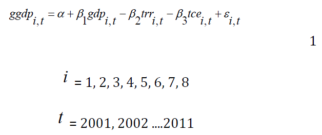
By this formula we can constructed an equation for penal data

Where, Green gross domestic product (), Gross domestic product (), Total natural resources rents (), Total cost of emissions (). stand for the cross sectional units and stand for the t^th time periods, is a deterministic constant factor and is a mean zero covariance stationary process and if the estimated value of is stationary significant then GDP and Green GDP trends of South Asian Country can forecast.

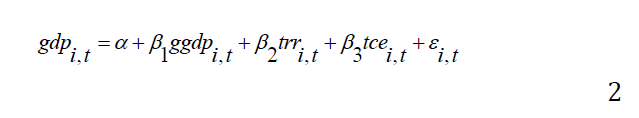
We can rewrite equation (2) as:

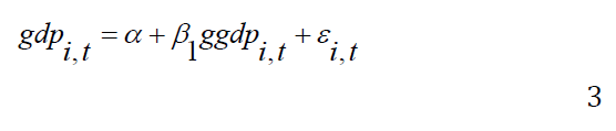
By limiting, the researcher is going to show impact of Green GDP on GDP for forecasting sustainable development. So the panel data model will be:

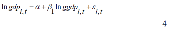
Now, by taking natural log in both sides we have

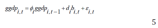
In this section, we investigate whether there is a long-run relationship between GDP and Green GDP. To do so, the researcher conduct recently developed panel data unit roots for data stationary and co-integration tests. The unit root tests of panel data are an augment of the univariate time series of unit root tests. The univariate unit root tests can’t easily reject null hypo-paper of panel data unit root approach. Now, Assuming the simple panel data model for Green GDP () with autoregressive AR (1) process.

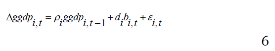
Where: = 1, 2, 3, ……, is the cross-section dimension, = 1, 2, 3, ……, is the time dimension, is a stationary error term the term may contain vector of panel –specific means and time trend or nothing, depending on the options specified in the panel unit root test and indicates corresponding vector of coefficients of . Equation (6) can be expressed as:

Therefore, the null hypothesis is := for all and the alternative hypopaper :<. In this paper Im-Pesaran-Shin (IPS) test use for individual unit root test.

The IPS Test

The IPS tests present mean of panel unit roots test designed against the homogeneous panel. Now, the econometrics model for the test of IPS for each cross section ADF regression model is:

Where the null hypothesis is : = for all and the alternative hypothesis gives permits some panel to have unit toots which is:

The group-mean -bar statistic can be constructed as the average of the individual augmented Dickey-Fuller statistics as follows:

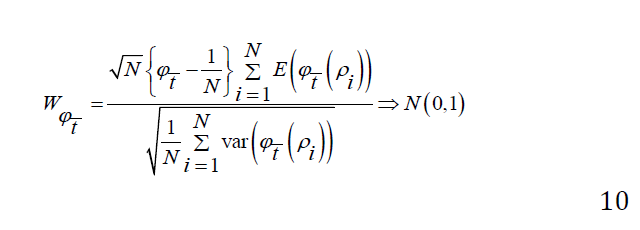
Where is the individual –statistic for testing : = , after adjustment for mean and variance for all in (8) and denote lag lengths. In the general case where for some cross-sections, [8], shows that a standardized has an asymptotic standard normal distribution:

Where, mean and variance of the ADF regression -statistics, and, are provided by [8], for various values of and. has standard normal limiting distribution as followed by while very negative values generate disbelief in .

Pedroni Test

Pedroni [1], suggested seven different residual-based panel cointegration tests for testing the null hypothesis of no cointegration. The four Within-dimension-based (i.e. panel- v, panel-, semi-parametric panel- t and parametric panel- t) statistics are calculated by summing up the numerator and the denominator over N cross-sections separately. The three between dimension-based (i.e. group-, semi-parametric group- and parametric- t) statistics are calculated by dividing the numerator and the before summing up over N cross-sections.

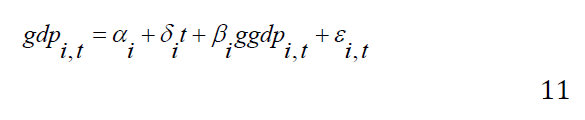
The Pedeoni [1], cointegration regression model is:

Where, = 1, 2, 3, …… , is the cross-section dimension, = 1, 2, 3, …… , is the time dimension, is a stationary error term and the dependent variable and dimensional vector of independent variables are assumed. The cointegration vectors the individual intercept and the trend parameter of cross-sections.

The null hypothesis of no cointegration for the panel cointegration test is the same for each statistic,

Whereas the alternative hypothesis for the between-dimension based and within-dimension based panel cointegration tests differ. The alternative hypothesis for the between-dimension-based statistics is

Source of Data, Calculation and Processing

All the data of South Asian Country were obtained from World Development Indicators (WDI) which published by World Bank (WB) for the periods of 2001 to 2011. For better calculation numerical value of GDP, total natural resources rent (the numerical value of GDP and natural resources rent directly obtain from WDI) and emission only consider Greenhouse Gas (GHG) the emission of carbon dioxide (CO2) are turn numerical value of $22.8 for per metric ton which proposed by Fankhauser in 1994 [9], (Fankhauser actually proposed a cost that rises over time: $22.8 for 2001-2010 and $25.3 for 2011-2020, the damage costs are increasing by $2.5 per metric ton for per decade). After all the data convert into numerical value then converted data into natural log. For calculating the result determination of optimal lag lengths used Akaike Information Criterion (AIC) with maximum lag length, bandwidth selection by Newey-West and kernel estimation by Bartlett automatically selected by Eviews software 7.

Empirical Results

In this paper used IPS to find out that the data are stationary or not and also used panel cointegration test Pedroni [1], for find out long run relationship between dependent in independent variables.

The Result of Panel Unit Root Test

The results of panel unit root test IPS without trend and with trend are explained below by table number 1 and 2.

According to Table 1, the panels data unit root test IPS provide empirical evidences that and are stationary at first difference at 1% significant level with individual intercept. So, easily can say according to the result IPS test rejects null hypothesis that panel data has unit root with common and individual unit root process and accept the alternative hypothesis that panel has not unit root or stationary. According to the result all panel are stationary that for mean, variance, are all constant over time and forecasting can made with significance.

According to Table 2, the panels data unit root test IPS also provide some empirical evidence that and are stationary at first difference at 10% significant level with individual intercept and trend. So, easily can say IPS test rejects null hypothesis that panel data has unit root with common and individual unit root process and accept the alternative hypothesis that panel data reduced unit root or stationary. 

Table 1: Panel Unit Root Test Results: (Without Trend)

Variable	Method	Level	First difference
LNGDP	IPS test	5.51480	-4.79496***
LNGGDP	IPS test	5.26721	-4.88495***

For determination of optimal lag lengths used Akaike Information Criterion (AIC) with maximum lag length, bandwidth selection by Newey-West and kernel estimation by Bartlett automatically selected by Eviews software 7. (***, ** and * show level of significance at 1%, 5% and 10%, respectively)

Table 2: Panel Unit Root Test Results: (With Trend)

Variable	Method	Level	First difference
LNGDP	IPS test	-0.36196	-1.33920*
LNGGDP	IPS test	-0.50978	-1.46252*

For determination of optimal lag lengths used Akaike Information Criterion (AIC) with maximum lag length, bandwidth selection by Newey-West and kernel estimation by Bartlett automatically selected by Eviews software 7. (***, ** and * show level of significance at 1%, 5% and 10%, respectively)

Panel Co-Integration Test Result

For find out panel cointegration, used Pedroni cointegration test for long run relationship between dependent and independent variable and Phillips-peron test for cross section specific result to find out individual relationship between dependent and independent variable. The results of the test are explained below by table number 3 and 4.

According to table 3, Pedroni [1], cointegration tests provide empirical evidence with individual intercept, individual intercept and individual trend test statistic within-dimension and between-dimension four test statistics, Panel PP-Statistic, Panel ADF-Statistic, Group PP-Statistic, Group ADF-Statistic are significance at 1% significant level but three test statistics Panel v-Statistic, Panel rho-Statistic, Group rho-Statistic are not significance at 1%, 5% or 10% significant level. According to the result out of seven, four statistics are significance at 1% significant level so, easily can say that between and have long run cointegration relationship.

Table 3: Pedroni [1], Cointegration Tests

For determination of optimal lag lengths used Akaike Information Criterion (AIC) with maximum lag length, bandwidth selection by Newey-West and kernel estimation by Bartlett automatically selected by Eviews software 7. (***, ** and * show level of significance at 1%, 5% and 10%, respectively)

According to table 4, shows individual cross section correlation result. The correlation bandwidth without trend indicates most of the country Afghanistan, Bangladesh, Pakistan, Sri Lanka bandwidth is 1, Bhutan bandwidth is 2 but India, Maldives, Nepal all three country correlations bandwidth is equal 9 that shows all the country of South Asia have correlation between variables of and in long run. In case of with trend cross section correlation bandwidth result of Afghanistan, Pakistan, Sri Lanka is 1, Bangladesh and India bandwidth is 4, Maldives bandwidth is 6, Bhutan and Nepal bandwidth is equal 9, that means with trend and without trend bandwidth correlation result of South Asian counters implies that there are correlation between and in long run.

Table 4: Phillips-Peron Cross Section Specific Result

For determination of optimal lag lengths used Akaike Information Criterion (AIC) with maximum lag length, bandwidth selection by Newey-West and kernel estimation by Bartlett automatically selected by Eviews software 7

This paper empirically analyzes the long run relationship between Green GDP and traditional GDP for forecasting sustainable development of South Asian country. For analysis the long run relationship uses panel data for the periods of 2001 to 2011. The study of 11 year periods uses autoregressive distributed lag model by panel unit root and cointegration test (panel unit root test LLC and IPS) for data stationary test and Pedroni [1], for data cointegration test. The results fiend out that most of the country of South Asia correlation bandwidth with and without trend are one or more than one except two country correlation bandwidth with trend are zero. The result also implies that GDP and Green GDP have long run relationship which shown Green GDP has significant impact on GDP and sustainable development. If South Asian country increase GDP without any kinds of environment damage that lead to greater increase in Green GDP. Which will promote better environment, biodiversity and ecology those are sign of sustainable development. South Asian country and global leaders should develop an appropriate accounting system for environmental valuation so, that the negative externality of environment can reduce.

This paper makes an attempt to calculate Green GDP from GDP as environmental valuation toward sustainable development. For the, future researchers could incorporate more comprehensive data and improve the result evaluation methodology for more accurate result for the sustainable development of South Asian region. 

Acknowledgment

First of all, we remember Almighty Allah for making us successful to complete the work. we would never have been able to conduct this paper without the blessings of the Almighty Allah, the most gracious and the most merciful. we praise the Almighty for providing this opportunity and strength to proceed successfully.

We gratefully acknowledge the hospitality and support of the Department of Economics at Bangladesh University of Business and Technology (BUBT). Lastly, we would like to state our thanks to the authors, researchers, whose books and articles we consulted.

1. Pedroni, P. “Panel cointegration: Asymptotic and finite sample properties of pooled time series test, with an application to the PPP hypopaper.” Econometric Theory, vol. 20, 2004, pp.575–625.

2. Theophile, A. et al. “Economic development and CO2 emissions: A nonparametric panel approach.” Discussion Paper, no. 05-56, 2005.

3. Talberth, J. and A.K. Bohara. “Economic openness and green GDP.” Ecological Economics, vol. 58, 2006, pp.743–758.

4. Sundas, K. and Khalid Z. “Climate change, green growth and sustainable development: A roadmap for sustainable SAARC region.” Journal of Economic Info, vol. 2, no. 1, 2014, pp.25–36.

5. Wawan, R. et al. “Assessment of green total factor productivity impact on sustainable indonesia productivity growth.” Procedia Environmental Sciences, vol. 28, 2015, pp.493–501.

6. Rahim, A.S. and Noraida A.W. “Modeling and forecasting the Malaysian GDP and green GDP: A comparative analysis.” The Fifth Congress of the East Asian Association of Environmental and Resource Economics, August 2015.

7. Negin, V. et al. “Green GDP and sustainable development in Malaysia.” Current World Environment, vol. 10, no. 1, 2015, pp.1–8.

8. Im, K.S. et al. “Testing for unit roots in heterogeneous panels.” Journal of Econometrics, vol. 115, 2003, pp.53–74.

9. Fankhauser, S. “Evaluating the social costs of greenhouse gas emissions.” The Energy Journal, vol. 15, no. 2, 1994, pp.157–184.